Решаем систему линейных алгебраических уравнений с python-пакетом scipy.linalg (не путать с numpy.linalg)

Length:

Return the specified unit in meters (e.g. returns )

Example

from scipy import constants

print(constants.inch)              #0.0254
print(constants.foot)              #0.30479999999999996
print(constants.yard)              #0.9143999999999999
print(constants.mile)              #1609.3439999999998
print(constants.mil)               #2.5399999999999997e-05
print(constants.pt)                #0.00035277777777777776
print(constants.point)             #0.00035277777777777776
print(constants.survey_foot)       #0.3048006096012192
print(constants.survey_mile)       #1609.3472186944373
print(constants.nautical_mile)     #1852.0
print(constants.fermi)             #1e-15
print(constants.angstrom)          #1e-10
print(constants.micron)            #1e-06
print(constants.au)                #149597870691.0
print(constants.astronomical_unit) #149597870691.0
print(constants.light_year)        #9460730472580800.0
print(constants.parsec)            #3.0856775813057292e+16

SciPy Interpolation

Interpolation is the process of estimating unknown values that fall between known values.SciPy provides us with a sub-package scipy.interpolation which makes this task easy for us. Using this package, we can perform 1-D or univariate interpolation and Multivariate interpolation. Multivariate interpolation (spatial interpolation ) is a kind interpolation on functions that consist of more than one variables. 

Here is an example of 1-D interpolation where there is only variable i.e. ‘x’:

First, we will define some points and plot them

import numpy as np  
from scipy import interpolate  
import matplotlib.pyplot as plt  
x = np.linspace(0, 5, 10)  
y = np.cos(x**2/3+4) 
plt.scatter(x,y,c='r')  
plt.show()  

Output:

scipy.interpolation provides interp1d class which is a useful method to create a function based on fixed data points. We will create two such functions that use different techniques of interpolation. The difference will be clear to you when you see the plotted graph of both of these functions.

from scipy.interpolate import interp1d  
import matplotlib.pyplot as plt  
fun1 = interp1d(x, y,kind = 'linear')  
fun2 = interp1d(x, y, kind = 'cubic')  
#we define a new set of input
xnew = np.linspace(0, 4,30)  
plt.plot(x, y, 'o', xnew, fun1(xnew), '-', xnew, fun2(xnew), '--')  
plt.legend(, loc = 'best')  
plt.show()

Output:

In the above program, we have created two functions fun1 and fun2. The variable x contains the sample points, and variable y contains the corresponding values. The third variable kind represents the types of interpolation techniques. There are various methods of interpolation. These methods are the following:

• Linear
• Nearest
• Zero
• S-linear
• Quadratic
• Cubic

Now what happens when we change the input values

from scipy.interpolate import interp1d  
import matplotlib.pyplot as plt  
fun1 = interp1d(x, y,kind = 'linear')  
fun2 = interp1d(x, y, kind = 'cubic')  
xnew = np.linspace(3, 5,30)  
plt.plot(x, y, 'o', xnew, fun1(xnew), '-', xnew, fun2(xnew), '--')  
plt.legend(, loc = 'best')  
plt.show()  

Output:

SciPy Cluster

Clustering is the task of dividing the population or data points into a number of groups such that data points in the same groups are more similar to other data points in the same group and dissimilar to the data points in other groups. Each group which is formed from clustering is known as a cluster. There are two types of the cluster, which are:

• Central
• Hierarchy

Here we will see how to implement the K-means clustering algorithm which is one of the popular clustering algorithms. The k-means algorithm adjusts the classification of the observations into clusters and updates the cluster centroids until the position of the centroids is stable over successive iterations.

In the below implementation, we have used NumPy to generate two sets of random points. After joining both these sets, we whiten the data. Whitening normalizes the data and is an essential step before using k-means clustering. Finally, we use the kmeans functions and pass it the data and number of clustered we want.

import numpy as np
from scipy.cluster.vq import  kmeans, whiten
import matplotlib.pyplot as plt
import seaborn as sns
sns.set_style("darkgrid")
# Create 50 datapoints in two clusters a and b
pts = 100
a = np.random.multivariate_normal(, 
                                  , ], 
                                  size=pts)
b = np.random.multivariate_normal(,
                                  , ],
                                  size=pts)
features = np.concatenate((a, b))
# Whiten data
whitened = whiten(features)
# Find 2 clusters in the data
codebook, distortion = kmeans(whitened, 2)
# Plot whitened data and cluster centers in red
plt.scatter(whitened, whitened)
plt.scatter(codebook, codebook, c='r')
plt.show()

Output:

SciPy linalg

SciPy has very fast linear algebra capabilities as it is built using the optimized ATLAS (Automatically Tuned Linear Algebra Software), LAPACK(Linear Algebra Package) and BLAS(Basic Linear Algebra Subprograms) libraries. All of these linear algebra routines can operate on an object that can be converted into a two-dimensional array and also returns the output as a two-dimensional array.

You might wonder that numpy.linalg also provides us with functions that help to solve algebraic equations, so should we use numpy.linalg or scipy.linalg? The scipy.linalg contains all the functions that are in numpy.linalg, in addition it also has some other advanced functions that are not in numpy.linalg. Another advantage of using scipy.linalg over numpy.linalg is that it is always compiled with BLAS/LAPACK support, while for NumPy this is optional, so it’s faster as mentioned before.

Solve Linear Equations

We can use scipy.linalg.solve() to solve a linear equation, all we need to know is how to represent our equations in terms of vectors. Here is an example:

import numpy as np  
from scipy import linalg  
# We are trying to solve a linear algebra system which can be given as   
#         x + 2y - 3z = -3 
#         2x - 5y + 4z = 13  
#         5x + 4y - z = 5  
#We will find values of x,y and z for which all these equations are zero
#Also finally we will check if the values are right by substituting them
#in the equations
# Creating input array  
a = np.array(, , ])  
# Solution Array  
b = np.array(, , ])  
# Solve the linear algebra  
x = linalg.solve(a, b)  
# Print results  
print(x)  
# Checking Results  
print("\n Checking results,must be zeros")  
print(a.dot(x) - b)  

As we can see, we got three values i.e 2,-1 and 1.So for x=2,y=-1 and z=1 the above three equations are zero as shown above.

Finding a determinant of a square matrix 

The determinant is a scalar value that can be computed from the elements of a square matrix and encodes certain properties of the linear transformation described by the matrix. The determinant of a matrix A is denoted det, det A, or |A|. In SciPy, this is computed using the det() function. It takes a matrix as input and returns a scalar value.

#importing the scipy and numpy packages
from scipy import linalg
import numpy as np
 
#Declaring the numpy array
A = np.array(,,])
#Passing the values to the det function
x = linalg.det(A)
 
#printing the result
print('Determinant of \n{} \n is {}'.format(A,x))

Eigenvalues and Eigenvectors

For a square matrix(A) we can find the eigenvalues (λ) and the corresponding eigenvectors (v) of by considering the following relation

We can use scipy.linalg.eig to computes the eigenvalues and the eigenvectors for a particular matrix as shown below:

#importing the scipy and numpy packages
from scipy import linalg
import numpy as np
 
#Declaring the numpy array
A = np.array(,,])
 
#Passing the values to the eig function
values, vectors = linalg.eig(A)
 
#printing the result for eigenvalues
print(values)
 
#printing the result for eigenvectors
print(vectors)

Linear Algebra with SciPy

• Linear Algebra of SciPy is an implementation of BLAS and ATLAS LAPACK libraries.
• Performance of Linear Algebra is very fast compared to BLAS and LAPACK.
• Linear algebra routine accepts two-dimensional array object and output is also a two-dimensional array.

Now let’s do some test with scipy.linalg,

Calculating determinant of a two-dimensional matrix,

from scipy import linalg
import numpy as np
#define square matrix
two_d_array = np.array(,  ])
#pass values to det() function
linalg.det( two_d_array )

Output: -7.0

Inverse Matrix –

scipy.linalg.inv()

Inverse Matrix of Scipy calculates the inverse of any square matrix.

Let’s see,

from scipy import linalg
import numpy as np
# define square matrix
two_d_array = np.array(,  ])
#pass value to function inv()
linalg.inv( two_d_array )

Output:

array( ,
       ] )

Eigenvalues and Eigenvector

scipy.linalg.eig()

• The most common problem in linear algebra is eigenvalues and eigenvector which can be easily solved using eig() function.
• Now lets we find the Eigenvalue of (X) and correspond eigenvector of a two-dimensional square matrix.

Example

from scipy import linalg
import numpy as np
#define two dimensional array
arr = np.array(,])
#pass value into function
eg_val, eg_vect = linalg.eig(arr)
#get eigenvalues
print(eg_val)
#get eigenvectors
print(eg_vect)

Output:

 #eigenvalues
  #eigenvectors
    ]

Почему SciPy?

SciPy предоставляет высокоуровневые команды и классы для управления данными и визуализации данных, что значительно увеличивает мощность интерактивного сеанса Python.

Помимо математических алгоритмов в SciPy, программисту доступно все, от классов, веб-подпрограмм и баз данных до параллельного программирования, что упрощает и ускоряет разработку сложных и специализированных приложений.

Поскольку SciPy имеет открытый исходный код, разработчики по всему миру могут вносить свой вклад в разработку дополнительных модулей, что очень полезно для научных приложений, использующих SciPy.

SciPy IO (Input & Output)

The functions provided by the scipy.io package enables us to work around with different formats of files such as:

• Matlab
• IDL
• Matrix Market
• Wave
• Arff
• Netcdf, etc.

The functions such as loadmat(), savemat() and whosmat() can load a MATLAB file, save a MATLAB file and list variables in a MATLAB file respectively. Here is an example:

First, save a MatLab file as test.mat which contains a structure as shown below:

Now we can use loadmat()  function to import this file into a python script as shown below:

from scipy.io import loadmat
x = loadmat('test.mat')
#save the individual elements as python object
lon = x
lat = x
# one-liner to read a single variable
lon = loadmat('test.mat')

Discrete Fourier Transform – scipy.fftpack

• DFT is a mathematical technique which is used in converting spatial data into frequency data.
• FFT (Fast Fourier Transformation) is an algorithm for computing DFT
• FFT is applied to a multidimensional array.
• Frequency defines the number of signal or wavelength in particular time period.

Example: Take a wave and show using Matplotlib library. we take simple periodic function example of sin(20 × 2πt)

%matplotlib inline
from matplotlib import pyplot as plt
import numpy as np 

#Frequency in terms of Hertz
fre  = 5 
#Sample rate
fre_samp = 50
t = np.linspace(0, 2, 2 * fre_samp, endpoint = False )
a = np.sin(fre  * 2 * np.pi * t)
figure, axis = plt.subplots()
axis.plot(t, a)
axis.set_xlabel ('Time (s)')
axis.set_ylabel ('Signal amplitude')
plt.show()

Output:

You can see this. Frequency is 5 Hz and its signal repeats in 1/5 seconds – it’s call as a particular time period.

Now let us use this sinusoid wave with the help of DFT application.

from scipy import fftpack

A = fftpack.fft(a)
frequency = fftpack.fftfreq(len(a)) * fre_samp
figure, axis = plt.subplots()

axis.stem(frequency, np.abs(A))
axis.set_xlabel('Frequency in Hz')
axis.set_ylabel('Frequency Spectrum Magnitude')
axis.set_xlim(-fre_samp / 2, fre_samp/ 2)
axis.set_ylim(-5, 110)
plt.show()

Output:

• You can clearly see that output is a one-dimensional array.
• Input containing complex values are zero except two points.
• In DFT example we visualize the magnitude of the signal.

Special Functions of Python SciPy

The following is the list of some of the most commonly used Special functions from the package of SciPy:

• Cubic Root
• Exponential Function
• Log-Sum Exponential Function
• Gamma

1. Cubic Root

The function is used to provide the element-wise cube root of the inputs provided.

Example:

from scipy.special import cbrt
val = cbrt()
print(val)

Output:

2. Exponential Function

The function is used to calculate the element-wise exponent of the given inputs.

Example:

from scipy.special import exp10
val = exp10()
print(val)

Output:

3. Log-Sum Exponential Function

The function is used to calculate the logarithmic value of the sum of the exponents of the input elements.

Example:

from scipy.special import logsumexp
import numpy as np
inp = np.arange(5)
val = logsumexp(inp)
print(val)

Here, numpy.arange() function is used to generate a sequence of numbers to be passed as input.

Output:

4.451914395937593

4. Gamma Function

Gamma function is used to calculate the gamma value, referred to as generalized factorial because, gamma(n+1) = n!

The function is used to calculate the gamma value of the input element.

Example:

from scipy.special import gamma
val = gamma()
print(val)

Output:

Special Function package

• scipy.special package contains numerous functions of mathematical physics.
• SciPy special function includes Cubic Root, Exponential, Log sum Exponential, Lambert, Permutation and Combinations, Gamma, Bessel, hypergeometric, Kelvin, beta, parabolic cylinder, Relative Error Exponential, etc..
• For one line description all of these function, type in Python console:

help(scipy.special)	
Output : 
NAME
    scipy.special

DESCRIPTION
    ========================================
    Special functions (:mod:`scipy.special`)
    ========================================
     
    .. module:: scipy.special
     
    Nearly all of the functions below are universal functions and follow
    broadcasting and automatic array-looping rules. Exceptions are noted.

Cubic Root Function:

Cubic Root function finds the cube root of values.

Syntax:

scipy.special.cbrt(x)

Example:

from scipy.special import cbrt
#Find cubic root of 27 & 64 using cbrt() function
cb = cbrt()
#print value of cb
print(cb)

Output: array()

Exponential Function:

Exponential function computes the 10**x element-wise.

Example:

from scipy.special import exp10
#define exp10 function and pass value in its
exp = exp10()
print(exp)

Output:

Permutations & Combinations:

SciPy also gives functionality to calculate Permutations and Combinations.

Combinations – scipy.special.comb(N,k)

Example:

from scipy.special import comb
#find combinations of 5, 2 values using comb(N, k)
com = comb(5, 2, exact = False, repetition=True)
print(com)

Output: 15.0

Permutations –

scipy.special.perm(N,k)

Example:

from scipy.special import perm
#find permutation of 5, 2 using perm (N, k) function
per = perm(5, 2, exact = True)
print(per)

Output: 20

Log Sum Exponential computes the log of sum exponential input element.

Syntax :

scipy.special.logsumexp(x) 

SciPy integrate

The integrate sub package of the Scipy package contains a lot of functions that allow us to calculate the integral of some complex functions. If you use the help function, you will find all the different types of integrals you can calculate. Here is how:

help(integrate)

So as you can see we have a wide variety of functions, now let us use a few of them here:

Single Integrals:

We use the quad function to calculate the single integral of a function. Numerical integrate is sometimes called quadrature and hence the name quad. The function has three parameters:

Here is an example where we use this function:

First, let us define a function using lambda function as shown below:

from numpy import exp  
f= lambda x:exp(-x**2)  

Remember, quad() function expects us to pass a function, thus we used lambda to form a function rather than using an expression.Now to calculate the integral:

import scipy 
i = scipy.integrate.quad(f, 0, 1)  
print(i)  

The first value is the tuple is the integral value with upper limit one and lower limit zero.Also, the second value is an estimate of the absolute error in the value of an integer.

Multiple Integrals

There are various functions such as dblquad(), tplquad(), and nquad() that enable us to calculate multiple integrals.the dblquad() function and tplquad() functions calculate the double and triple integrals respectively,whereas nquad performs n-fold multiple integration.

Below we will use scipy.integrate.dblquad(func,a,b,gfun,hfun) to solve double integrals. The first argument func is the name of the function to be integrated and a and b are the lower and upper limit of the x variable.  While gfun and hfun are names of the functions that define the lower and upper limit of the y variable.It is important to note that that limits of inner integrals must be passed functions as in the following example:

import scipy.integrate  
from numpy import exp  
from math import sqrt  
f = lambda x, y : 2*x*y  
g = lambda x : 0  
h = lambda y : 4*y**2  
i = scipy.integrate.dblquad(f, 0, 0.5, g, h)  
print(i)

1.6.5. Optimization and fit: scipy.optimize¶

Optimization is the problem of finding a numerical solution to a
minimization or equality.

Tip

The module provides algorithms for function
minimization (scalar or multi-dimensional), curve fitting and root
finding.

>>> from scipy import optimize

1.6.5.1. Curve fitting

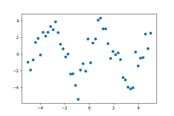
Suppose we have data on a sine wave, with some noise:

>>> x_data = np.linspace(-5, 5, num=50)
>>> y_data = 2.9 * np.sin(1.5 * x_data) + np.random.normal(size=50)

If we know that the data lies on a sine wave, but not the amplitudes
or the period, we can find those by least squares curve fitting. First we
have to define the test function to fit, here a sine with unknown
amplitude and period:

>>> def test_func(x, a, b):
...     return a * np.sin(b * x)

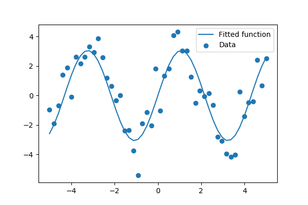
We then use to find and :

>>> params, params_covariance = optimize.curve_fit(test_func, x_data, y_data, p0=2, 2])
>>> print(params)

Exercise: Curve fitting of temperature data

1.6.5.2. Finding the minimum of a scalar function

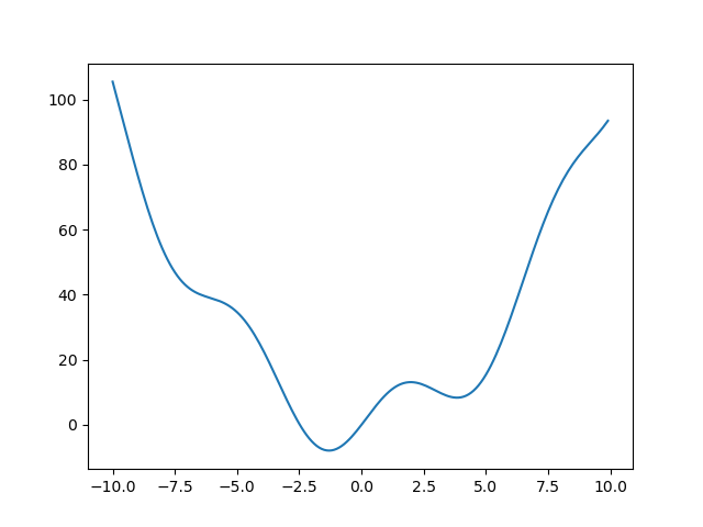
Let’s define the following function:

>>> def f(x):
...     return x**2 + 10*np.sin(x)

and plot it:

>>> x = np.arange(-10, 10, 0.1)
>>> plt.plot(x, f(x)) 
>>> plt.show() 

This function has a global minimum around -1.3 and a local minimum around
3.8.

Searching for minimum can be done with
, given a starting point x0, it returns
the location of the minimum that it has found:

result type

The result of is a compound object
comprising all information on the convergence

>>> result = optimize.minimize(f, x0=)
>>> result 
      fun: -7.9458233756...
 hess_inv: array(`0`.`0858`.``.``.``)
      jac: array()
  message: 'Optimization terminated successfully.'
     nfev: 18
      nit: 5
     njev: 6
   status: 0
  success: True
        x: array()
>>> result.x # The coordinate of the minimum  
array()

Methods:
As the function is a smooth function, gradient-descent based methods are
good options. The lBFGS algorithm is a good choice
in general:

>>> optimize.minimize(f, x0=, method="L-BFGS-B")  
      fun: array()
 hess_inv: <1x1 LbfgsInvHessProduct with dtype=float64>
      jac: array()
  message: ...'CONVERGENCE: NORM_OF_PROJECTED_GRADIENT_<=_PGTOL'
     nfev: 12
      nit: 5
   status: 0
  success: True
        x: array()

Note how it cost only 12 functions evaluation above to find a good value
for the minimum.

Global minimum:
A possible issue with this approach is that, if the function has local minima,
the algorithm may find these local minima instead of the
global minimum depending on the initial point x0:

>>> res = optimize.minimize(f, x0=3, method="L-BFGS-B")
>>> res.x
array()

If we don’t know the neighborhood of the global minimum to choose the
initial point, we need to resort to costlier global optimization. To
find the global minimum, we use
(added in version 0.12.0 of Scipy). It combines a local optimizer with
sampling of starting points:

>>> optimize.basinhopping(f, )  
                  nfev: 1725
 minimization_failures: 0
                   fun: -7.9458233756152845
                     x: array()
               message: 
                  njev: 575
                   nit: 100

Note

used to contain the routine anneal, it has been removed in
SciPy 0.16.0.

Constraints:
We can constrain the variable to the interval
using the “bounds” argument:

A list of bounds

As works in general with x
multidimensionsal, the “bounds” argument is a list of bound on each
dimension.

>>> res = optimize.minimize(f, x0=1,
...                         bounds=((, 10), ))
>>> res.x    
array()

Tip

What has happened? Why are we finding 0, which is not a mimimum of our
function.

Minimizing functions of several variables

To minimize over several variables, the trick is to turn them into a
function of a multi-dimensional variable (a vector). See for instance
the exercise on 2D minimization below.

Note

is a function with dedicated
methods to minimize functions of only one variable.

See also

Finding minima of function is discussed in more details in the
advanced chapter: .

Exercise: 2-D minimization

SciPy ODR

Orthogonal Distance Regression (ODR) is the name given to the computational problem associated with finding the maximum likelihood estimators of parameters in measurement error models in the case of normally distributed errors.

The Least square method calculates the error vertical to the line (shown by grey colour here) whereas ODR calculates the error perpendicular(orthogonal) to the line. This accounts for the error in both X and Y whereas using  Least square method, we only consider the error in Y.

scipy.odr Implementation for Univariate Regression

import numpy as np
import scipy.odr.odrpack as odrpack
np.random.seed(1)

N = 100
x = np.linspace(0,10,N)
y = 3*x - 1 + np.random.random(N)
sx = np.random.random(N)
sy = np.random.random(N)

def f(B, x):
    return B*x + B
linear = odrpack.Model(f)
# mydata = odrpack.Data(x, y, wd=1./np.power(sx,2), we=1./np.power(sy,2))
mydata = odrpack.RealData(x, y, sx=sx, sy=sy)

myodr = odrpack.ODR(mydata, linear, beta0=)
myoutput = myodr.run()
myoutput.pprint()

История

В 1990-х годах Python был расширен за счет включения в него типа массива для числовых вычислений под названием Numeric (этот пакет в конечном итоге был заменен Трэвисом Олифантом, который написал NumPy в 2006 году как смесь Numeric и Numarray, которая была начата в 2001 году). По состоянию на 2000 год росло число модулей расширения и возрастал интерес к созданию полноценной среды для научных и технических вычислений. В 2001 году Трэвис Олифант, Эрик Джонс и Пиару Петерсон объединили написанный ими код и назвали получившийся пакет SciPy. Вновь созданный пакет предоставляет стандартный набор общих числовых операций поверх структуры данных числового массива. Вскоре после этого Фернандо Перес выпустил IPython , расширенную интерактивную оболочку, широко используемую в сообществе технических вычислений, а Джон Хантер выпустил первую версию Matplotlib , библиотеки 2D-графиков для технических вычислений. С тех пор среда SciPy продолжала расти с появлением большего количества пакетов и инструментов для технических вычислений .

SciPy Ndimage

The SciPy provides the ndimage (n-dimensional image) package, that contains the number of general image processing and analysis functions. Some of the most common tasks in image processing are as follows:

• Basic manipulations − Cropping, flipping, rotating, etc.
• Image filtering − Denoising, sharpening, etc.
• Image segmentation − Labeling pixels corresponding to different objects
• Classification
• Feature extraction
• Registration

Here are some examples in which we will apply some of these image processing techniques on the images:

First, let us import an image that is already included in the SciPy package:

import scipy.misc
import matplotlib.pyplot as plt
face = scipy.misc.face()#returns an image of raccoon
#display image using matplotlib
plt.imshow(face)
plt.show()

Output:

Crop image

import scipy.misc
import matplotlib.pyplot as plt
face = scipy.misc.face()#returns an image of raccoon
lx,ly,channels= face.shape
# Cropping
crop_face = face[int(lx/4):int(-lx/4), int(ly/4):int(-ly/4)]
plt.imshow(crop_face)
plt.show()

Output:

Rotate Image

from scipy import misc,ndimage
import matplotlib.pyplot as plt
face = misc.face()
rotate_face = ndimage.rotate(face, 180)
plt.imshow(rotate_face)
plt.show()

Output:

Blurring or Smoothing  Images

Here we will blur the original images using the Gaussian filter and see how to control the level of smoothness using the sigma parameter.

from scipy import ndimage,misc
import matplotlib.pyplot as plt

face = scipy.misc.face(gray=True)
blurred_face = ndimage.gaussian_filter(face, sigma=3)
very_blurred = ndimage.gaussian_filter(face, sigma=5)

plt.figure(figsize=(9, 3))
plt.subplot(131)
plt.imshow(face, cmap=plt.cm.gray)
plt.axis('off')
plt.subplot(132)
plt.imshow(very_blurred, cmap=plt.cm.gray)
plt.axis('off')
plt.subplot(133)
plt.imshow(blurred_face, cmap=plt.cm.gray)
plt.axis('off')


plt.subplots_adjust(wspace=0, hspace=0., top=0.99, bottom=0.01,
                    left=0.01, right=0.99)

plt.show()

Output:

The first image is the original image followed by the blurred images with different sigma values.

Sharpening images

Here we will blur the image using the Gaussian method mentioned above and then sharpen the image by adding intensity to each pixel of the blurred image.

import scipy
from scipy import ndimage
import matplotlib.pyplot as plt

f = scipy.misc.face(gray=True).astype(float)
blurred_f = ndimage.gaussian_filter(f, 3)

filter_blurred_f = ndimage.gaussian_filter(blurred_f, 1)

alpha = 30
sharpened = blurred_f + alpha * (blurred_f - filter_blurred_f)

plt.figure(figsize=(12, 4))

plt.subplot(131)
plt.imshow(f, cmap=plt.cm.gray)
plt.axis('off')
plt.subplot(132)
plt.imshow(blurred_f, cmap=plt.cm.gray)
plt.axis('off')
plt.subplot(133)
plt.imshow(sharpened, cmap=plt.cm.gray)
plt.axis('off')

plt.tight_layout()
plt.show()

Output:

Edge detection

Edge detection includes a variety of mathematical methods that aim at identifying points in a digital image at which the image brightness changes sharply or, more formally, has discontinuities. The points at which image brightness changes sharply are typically organized into a set of curved line segments termed edges.

Here is an example where we make a square figure and then find its edges:

mport numpy as np
from scipy import ndimage
import matplotlib.pyplot as plt

im = np.zeros((256, 256))
im = 1

im = ndimage.rotate(im, 15, mode='constant')
im = ndimage.gaussian_filter(im, 8)

sx = ndimage.sobel(im, axis=0, mode='constant')
sy = ndimage.sobel(im, axis=1, mode='constant')
sob = np.hypot(sx, sy)

plt.figure(figsize=(9,5))
plt.subplot(141)
plt.imshow(im)
plt.axis('off')
plt.title('square', fontsize=20)
plt.subplot(142)
plt.imshow(sob)
plt.axis('off')
plt.title('Sobel filter', fontsize=20)
plt.show()

Output:

NumPy¶

There is now a journal article available for citing usage of NumPy:

Charles R. Harris, K. Jarrod Millman, Stéfan J. van der Walt, Ralf
Gommers, Pauli Virtanen, David Cournapeau, Eric Wieser, Julian Taylor,
Sebastian Berg, Nathaniel J. Smith, Robert Kern, Matti Picus, Stephan
Hoyer, Marten H. van Kerkwijk, Matthew Brett, Allan Haldane, Jaime
Fernández del Río, Mark Wiebe, Pearu Peterson, Pierre Gérard-Marchant,
Kevin Sheppard, Tyler Reddy, Warren Weckesser, Hameer Abbasi,
Christoph Gohlke & Travis E. Oliphant.
Array programming with NumPy, Nature, 585, 357–362 (2020),
DOI:10.1038/s41586-020-2649-2 (publisher link)

Here’s an example of a BibTeX entry:

Каковы особенности?

Библиотека ориентирована на моделирование данных. Он не ориентирован на загрузку, манипулирование и суммирование данных. Для этих функций, обратитесь к NumPy и Pandas.

Некоторые популярные группы моделей, предоставляемые Scikit-Learn, включают в себя:

• Кластеризация: для группировки немаркированных данных, таких как KMeans.
• Перекрестная проверка: для оценки производительности контролируемых моделей на невидимых данных.
• Datasets: для тестовых наборов данных и для создания наборов данных со специфическими свойствами для исследования поведения модели.
• Уменьшение размерности: для уменьшения количества атрибутов в данных для суммирования, визуализации и выбора функций, таких как анализ главных компонентов.
• Методы ансамбля: для объединения прогнозов нескольких контролируемых моделей.
• Извлечение функций: для определения атрибутов в графических и текстовых данных.
• Выбор функции: для определения значимых атрибутов, из которых можно создавать контролируемые модели.
• Настройка параметров: для получения максимальной отдачи от контролируемых моделей.
• Многообразие обучения: Для суммирования и отображения сложных многомерных данных.
• Модели под наблюдением: обширный массив, не ограниченный обобщенными линейными моделями, дискриминирующим анализом, наивными байесовскими алгоритмами, ленивыми методами, нейронными сетями, машинами опорных векторов и деревьями решений.

SciPy FFTpack

The FFT stands for Fast Fourier Transformation which is an algorithm for computing DFT. DFT is a mathematical technique which is used in converting spatial data into frequency data.

SciPy provides the fftpack module, which is used to calculate Fourier transformation. In the example below, we will plot a simple periodic function of sin and see how the scipy.fft function will transform it.

from matplotlib import pyplot as plt
import numpy as np 
import seaborn as sns
sns.set_style("darkgrid")
#Frequency in terms of Hertz
fre  = 10
#Sample rate
fre_samp = 100
t = np.linspace(0, 2, 2 * fre_samp, endpoint = False )
a = np.sin(fre  * 2 * np.pi * t)
plt.plot(t, a)
plt.xlabel('Time (s)')
plt.ylabel('Signal amplitude')
plt.show()

Output:

from scipy import fftpack
A = fftpack.fft(a)
frequency = fftpack.fftfreq(len(a)) * fre_samp
plt.stem(frequency, np.abs(A),use_line_collection=True)
plt.xlabel('Frequency in Hz')
plt.ylabel('Frequency Spectrum Magnitude')
plt.show()

Output:

This subpackage also provides us functions such as fftfreq() which will generate the sampling frequencies. Also fftpack.dct() function allows us to calculate the Discrete Cosine Transform (DCT).SciPy also provides the corresponding IDCT with the function idct().

Проверка на нормальность в Scipy

Нормальный закон распределения является простым и удобным для дальнейшего исследования. Чтобы проверить имеет ли тот или иной атрибут нормальное распределение, можно воспользоваться двумя критериями Python-библиотеки с модулем . Модуль   поддерживает большой диапазон статистических функций, полный перечень которых представлен в официальной документации.

В основе проверки на “нормальность” лежит проверка гипотез. Нулевая гипотеза – данные распределены нормально, альтернативная гипотеза – данные не имеют нормального распределения.

Проведем первый критерий Шапиро-Уилк [], возвращающий значение вычисленной статистики и p-значение. В качестве критического значения в большинстве случаев берется 0.05. При p-значении меньше 0.05 мы вынуждены отклонить нулевую гипотезу.

Проверим распределение атрибута Rings, количество колец:

import scipy

stat, p = scipy.stats.shapiro(data) # тест Шапиро-Уилк
print('Statistics=%.3f, p-value=%.3f' % (stat, p))

alpha = 0.05
if p > alpha:
    print('Принять гипотезу о нормальности')
else:
    print('Отклонить гипотезу о нормальности')

В результате мы получили низкое p-значение и, следовательно, отклоняем нулевую гипотезу:

Statistics=0.931, p-value=0.000
Отклонить гипотезу о нормальности

Второй тест по критерию согласия Пирсона [], который тоже возвращает соответствующее значение статистики и p-значение:

stat, p = scipy.stats.normaltest(data) # Критерий согласия Пирсона
print('Statistics=%.3f, p-value=%.3f' % (stat, p))

alpha = 0.05
if p > alpha:
    print('Принять гипотезу о нормальности')
else:
    print('Отклонить гипотезу о нормальности')

Этот критерий также отвергает нулевую гипотезу о нормальности распределения колец у моллюсков, так как p-значение меньше 0.05:

Statistics=242.159, p-value=0.000
Отклонить гипотезу о нормальности